

Hardy Weinberg Mathematical Model Worksheet Answers
Skip Nav Destination
Research Article | October 01 2017
Using Spreadsheets to Simulate an Evolving Population
Ryan E. Langendorf;
2RYAN E. LANGENDORF is a PhD candidate in Environmental Studies and Interdisciplinary Quantitative Biology at the University of Colorado at Boulder, 397 UCB, Boulder, Colorado 80309; email: ryan.langendorf@colorado.edu.
Search for other works by this author on:
Paul K. Strode
1PAUL K. STRODE is a biology teacher at Fairview High School in Boulder, Colorado.
Search for other works by this author on:
The American Biology Teacher (2017) 79 (8): 635–643.
Biology teachers inevitably struggle with how best to teach evolution. Students arrive in their classrooms with preconceptions, many of which are overwhelmingly skeptical, and science teachers are increasingly being pressured to adhere to an arbitrary degree of objectivity that makes discussing scientific worldviews challenging. These challenges have resulted in evolution being taught largely as a series of explanations for questions arising from observations of the living world. In so doing, students may not have a chance to grapple with the worldview that produced those explanations, or develop a more mechanistic intuition for inheritance and change in the world they see around themselves. Here we put forth all the tools necessary for a class to build a simulation of an evolving population experiencing natural selection from scratch in a Google Docs spreadsheet. Not only will this activity help students experiment with the natural world more mechanistically, but it will also allow them to learn as actual evolutionary biologists do.
Introduction
Evolutionary theory is the unifying paradigm for the life sciences, yet the underlying explanatory framework is the curricular topic met with the most resistance (Young & Strode, 2009). Even with confirmation from national science academies around the world (Panel, 2006) and support from the United States legal system deeming evolution the only scientific theory of life's history (e.g., Edwards v. Aguillard, 1987; Kitzmiller v. Dover Area School District, 2005), 42 percent of Americans polled in 2014 agreed with the statement, "God created human beings pretty much in their present form at one time within the last 10,000 years or so." (Newport, 2014). The result is that many students come to a biology classroom from a social context that prevents meaningful engagement with our current scientific understanding of the history of the natural world (Kahan et al., 2011). This social phenomenon is exacerbated by 73 percent of high school biology teachers themselves being either unsure how to teach evolution or actually endorsing creationism in the classroom (Berkman & Plutzer, 2011). These data suggest that evolution education requires new approaches.
Some of this disagreement and confusion may stem from focusing on adaptations as a well-meaning way to teach through evidence. Doing so injects a sense of intention into the history of life by giving students the impression that beneficial traits arise because they are needed. It also makes evolution more amenable to competing teleological explanations. Indeed, we have all had students make teleological claims: for example, that birds evolved wings so that they could fly. Rather than focusing in hindsight on the successes of evolution, it should be taught as a process, and one that is inherently stochastic (involving random elements over time; Bonner, 2013). Part of the difficulty, for teachers and students alike, is that much of the stochasticity occurs at unobservable spatial and temporal scales. This challenge leaves teachers struggling to span microscopic and macroscopic explanations of evolution in order to bridge the gap between what can be directly observed, like antibiotic resistance, and the more contentious large-scale results of evolution like speciation. Instead, students would benefit from experimenting themselves with the way simple inheritance mechanisms work.
Today's computing technology allows teachers and their students to simulate evolution as they could never have done before. If students are willing to sacrifice some computing power, such simulations can even be built from scratch in a spreadsheet program, allowing them to create their own knowledge much the same way scientists do. Here we detail one such simulation run in the free online program Google Docs, which relies on random numbers and allelic reproductive advantages to build a more realistically probabilistic intuition for the relationship between evolutionary mechanisms and outcomes. If scientific research is inherently an inquiry-based process, as John Dewey argued over a century ago (Herman & Pinard, 2015), our students should engage in the practice as an essential component of their science education. This is especially true for challenging topics like evolution.
Educational Goals
As represented in modern standards, science education is moving away from content-oriented lecturing and toward active learning and metacognition, where students construct their own knowledge through inquiry (Huffaker & Calvert, 2003; Niemi, 2002). This embracing of how scientists actually work is embodied by lessons such as this one, which emphasize individual knowledge creation in the manner of the field of evolutionary science itself. Accordingly, at the end of this lesson students will be able to (a) use statistics, probability, and basic programming skills to represent inheritance mechanisms and explain changes in trait frequencies over time, (b) use both simulated and real data to explain the roles of natural selection and genetic drift in a population's genetic makeup, and (c) make probabilistic predictions about a population (Table 1).
Table 1.
Referenced educational standards.
| Next Generation Science Standards (NGSS) | |
| HS-LS3-3 | Apply concepts of statistics and probability to explain the variation and distribution of expressed traits in a population. |
| HS-LS4-2 | Construct an explanation based on evidence that the process of evolution primarily results from four factors: (1) the potential for a species to increase in number, (2) the heritable genetic variation of individuals in a species due to mutation and sexual reproduction, (3) competition for limited resources, and (4) the proliferation of those organisms that are better able to survive and reproduce in the environment. |
| MS-LS4-6 | Use mathematical representations to support explanations of how natural selection may lead to increases and decreases of specific traits in populations over time. |
| AP Biology Learning Objectives | |
| 1.13 | The student is able to construct and/or justify mathematical models, diagrams or simulations that represent processes of biological evolution. |
| 1.25 | The student is able to describe a model that represents evolution within a population. |
| 1.6 | The student is able to use data from mathematical models based on the Hardy-Weinberg equilibrium to analyze genetic drift and effects of selection in the evolution of specific populations. |
| 1.7 | The student is able to justify data from mathematical models based on the Hardy-Weinberg equilibrium to analyze genetic drift and the effects of selection in the evolution of specific populations. |
| 1.3 | The student is able to apply mathematical methods to data from a real or simulated population to predict what will happen to the population in the future. |
| 1.8 | The student is able to make predictions about the effects of genetic drift, migration and artificial selection on the genetic makeup of a population. |
| 1.22 | The student is able to use data from a real or simulated population(s), based on graphs or models of types of selection, to predict what will happen to the population in the future. |
Lesson Guide
This activity was designed to help students explore the way genetics, chance, selection, and population size lead to changes in an evolving population. As such, it works best if the students are already familiar with each of these topics and their respective terminology. We recommend teaching it after evolution, at the end of a genetics unit. Additionally, we have had success in establishing motivation in students for this activity by first having the class interactively simulate the same process themselves, either in an abbreviated form at the start of the class or altogether in a previous class. We have used Lab 8 in the older 2001 AP Biology Lab Manual, which has students simulate several generations of a population by randomly exchanging cards with alleles on them, and recommend similar activities (Brewer & Gardner, 2013).
Starting with an interactive simulation helps students build an intuition for what their computer will have to do while illustrating the power of using computers to explore complicated dynamics that are not easily captured without lots of data. Alternatively, Investigation 2: Mathematical Modeling: Hardy-Weinberg in the current AP Biology Investigative Labs manual (within Big Idea 1: Evolution) teaches the same content using a pre-made spreadsheet simulation. This more detailed Hardy-Weinberg activity can be used in conjunction with the activity detailed here, either to offer students a chance to engage with the simulation at a more fundamental level, or to expand the activity into a larger unit covered by a traditional AP Biology course.
Logistically, the activity was designed to take place over two 50-minute periods, but it can also be reasonably taught in one longer period with the discussion questions at the end converted to a worksheet to be completed by students at home. Most importantly, students will need a computer with Internet access, but do not need more than one computer per group. The equations provided are specific to Google Sheets and will not all work correctly in other spreadsheet applications, such as Microsoft Excel or Apple Numbers. All Google Docs, including Sheets, are freely accessible online and easily saved and shared, so students can work on any computer and take their simulation with them afterward. We hope this will make the activity more widely usable for teachers and reusable for students.
The following links (shortened from their longer original Google URLs) make a copy of the source spreadsheets, which will stay active and static, so teachers and students can make as many copies of the original as they like:
-
Empty template (N = 10 individuals): http://tinyurl.com/EvolveSim-Template
-
Completed version (N = 10 individuals): http://tinyurl.com/EvolveSim-Completed
-
Completed version (N = 100 individuals): http://tinyurl.com/EvolveSim-Completed-Large
Day 1 (50 minutes)
The first day should be spent entirely on building the simulation, which is to be done by the students in small groups. The template spreadsheet helps by ensuring all of the functions work correctly to produce the final figure (see Figure 1, section 7), but there is no reason not to adapt the general concept to a different layout. Additionally, it is easier to work with a smaller population so everything can fit on a computer screen simultaneously, but the simulation really should be applied to more realistic population sizes. We have supplied a version with only 10 individuals, so students can see all 7 sections simultaneously and re-run the simulation many times very quickly, as well as a more realistic version with 100 individuals that takes longer to run, during which students can work on discussion questions. Unfortunately, larger population sizes (e.g., N = 1000) take too long to run after each change in the spreadsheet, making them unusable. For teachers more interested in the output of these kinds of simulations than actually building them, we recommend programs such as AlleleA1 (http://faculty.washington.edu/herronjc/SoftwareFolder/AlleleA1.html).
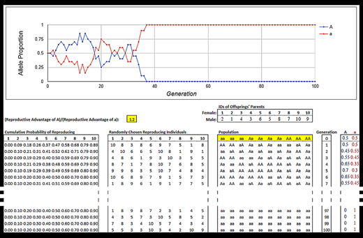
Figure 1.
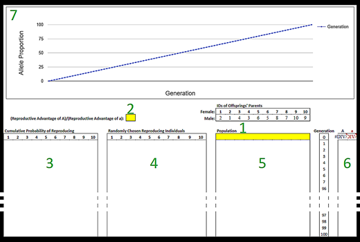
Layout of the simulation as it appears in the accompanying Google Sheets template (N = 10). Sections are labeled in the order they are to be completed by students: (1) starting population; (2) (reproductive advantage of A)/(reproductive advantage of a); (3) cumulative probability of reproducing; (4) randomly chosen reproducing individuals; (5) population; (6) allelic proportions; (7) graph of allelic proportions. Generations 6 through 96 are not shown to save space. Highlighted cells indicate where students can manipulate the simulation.
Figure 1.
Layout of the simulation as it appears in the accompanying Google Sheets template (N = 10). Sections are labeled in the order they are to be completed by students: (1) starting population; (2) (reproductive advantage of A)/(reproductive advantage of a); (3) cumulative probability of reproducing; (4) randomly chosen reproducing individuals; (5) population; (6) allelic proportions; (7) graph of allelic proportions. Generations 6 through 96 are not shown to save space. Highlighted cells indicate where students can manipulate the simulation.
Each section should be completed in the order it is listed in Figure 1 using the equations in Table 2. Correct completion of the simulation is important so that students can use it to answer questions about inheritance and selection, but no more so than the process of creating it. As such, students should fill in each section only after its literal function and its relation to the overarching goal of simulating an evolving population is discussed with the class. Doing so will help prevent students from getting lost, but also emphasizes the multistep nature of science where hypotheses are tested using complicated protocols involving both specific and holistic challenges.
Table 2.
Google Sheets equations. Each section's purpose is given, followed by equations for the upper left cell of each section, divided into conceptual pieces with accompanying explanations, and followed by discussion questions with italicized answers.
| Section | Explanations, Equations, and Questions |
|---|---|
| 1 | Starting Population: This row contains the genotypes of those individuals in the starting population, labelled generation 0. NO EQUATION. This is user-specified and is meant to be changed as a way of exploring different scenarios.
|
| 2 | (Reproductive Advantage of A)/(Reproductive Advantage of a): Determines how likely an individual with the dominant mutation A is to reproduce relative to a homozygous recessive aa individual. NO EQUATION. This is a user-specified number that is meant to be changed as a way of simulating natural selection. It can be any non-negative value, as large or small as you like.
|
| 3 | Cumulative Probability of Reproducing: Creates a cumulative probability distribution of the probability of each individual reproducing based on the specified Reproductive Advantage in Section 2. This is a mathematically convenient way of randomly selecting individuals when their probabilities of reproducing are not all the same. It does not refer to the way mutations accumulate over generations.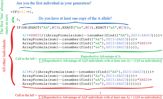
|
| 4 | Randomly Chosen Reproducing Individuals: Picks individuals to reproduce based on the probabilities assigned to each individual in the Cumulative Probability of Reproducing in section 3.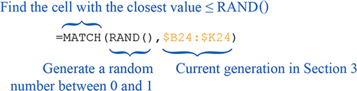
|
| 5 | Population: Randomly assigns one allele each from two randomly chosen individuals in the previous generation to create a new individual.
|
| 6 | Allelic Proportions: Calculates the population's allelic frequencies. Note that the columns have different equations.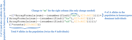
|
| 7 | Graph of Allelic Proportions: Visualizes the proportion of each allele in the population across all simulated generations. NO EQUATION. The figure will automatically appear after section 6 is completed. |
The equations provided should be entered in the upper left cell of the corresponding section. This cell can then be dragged to the right and down to fill in the entire section. Alternatively, as dragging cells can be tedious, quick cell filling can also be accomplished by highlighting all of the cells, including the upper left cell with the equation already entered, and then pressing Ctrl + R and then Ctrl + D. The reverse order (Ctrl + D followed by Ctrl + R) also works. Either method will also copy the borders on the upper left cell in each section. These borders have no effect on the contents of the cells and can be manually deleted.
The completed spreadsheet will then resemble Figure 2. Refreshing the spreadsheet (Ctrl + R) will automatically recalculate the entire evolutionary simulation, and redraw the final figure (section 7).
Figure 2.
An example of a completed simulation. Generations 8 through 96 are not shown to save space. Highlighted cells indicate where students can manipulate the simulation.
Figure 2.
An example of a completed simulation. Generations 8 through 96 are not shown to save space. Highlighted cells indicate where students can manipulate the simulation.
Day 2 (50 minutes)
Once the simulation is built, students can focus on using it to explore the relationships among inheritance, natural selection, and chance. We designed the following short-answer, multipart questions as examples for teachers to make this exploration creative and challenging, but also relevant to the previously stated educational goals. Their purpose is to stimulate discussions, either within small groups or as a class. The goal here is not for students to provide correct answers to every sub-question.
| Question 1. | Conservation biologists are concerned with preserving and promoting genetic diversity. What is the mean generation time for genetic drift to cause a neutral allele (no reproductive advantage or disadvantage) to become fixed in the population? If you were in charge of making decisions that would impact an endangered species, how helpful would this mean generation time be? What else might you want to know? Reasonable responses should address the idea that the mean alone is not a good basis for conservation decisions. Some sense of variability would allow for more informed action. |
| Question 2. | Genetic drift is an evolutionary mechanism known to cause populations to change from one generation to the next. How long does it take for genetic drift to cause the population to be significantly different in future generations from when it started, based on the allele frequencies? (Hint: The answer is different every time you run the simulation. How many generations are needed so that 50% of the time the population will be significantly different? 75%? 95%?) What statistical test should be used here? If you had to decide whether to classify a species as endangered, does it make sense to rely on statistical significance? Reasonable responses should address the difference between biological and statistical significance. The chi-square goodness-of-fit test addresses the latter, but effective conservation requires understanding that this is not always relevant because statistically significant effects can be so small that they are likely meaningless to the actual population. An easy to use chi-square goodness-of-fit test can be found here: http://turner.faculty.swau.edu/mathematics/math241/materials/contablecalc/. Students will have to convert their proportions back into the actual number of A and a alleles by multiplying the proportions by twice the size of the population (every individual has two alleles). |
| Question 3. | How much do the "starting conditions" (i.e., the allele frequencies in the starting generation) matter? How is an endangered species that used to be common different from a species that was never very numerous? Does the historical difference matter if both species are currently endangered? Reasonable responses should address the importance of the "starting conditions." Population bottlenecks (like what cheetahs went through) are so dangerous because even if the number of individuals increases, they will still have less genetic variability, just as if there were never many of them. Moreover, there is no difference between losing genetic variability and never having much in the first place. Moving forward, populations in both situations will struggle to adapt to a changing environment and selective pressures. |
| Question 4. | How much of a reproductive advantage does a mutation need to offer for it to become fixed in the population 50 percent of the time? Did you expect this to be larger? Smaller? Why? How might this depend on the size of the population? What about whether the mutation is dominant or recessive? How much of an advantage do most mutations likely offer? Reasonable responses should include the idea that it takes a very advantageous mutation or quite a bit of luck (or some combination) for a mutation to become fixed in the population. Additionally, students might comment on how this implies a fast rate of mutations, and how challenging it is for scientists to quantify the advantage or disadvantage of a single mutation. |
| Question 5. | This simulation is built entirely on manipulating random numbers. Where do random numbers come from? Are they actually random? Try to come up with a way of creating random numbers on your own. Reasonable responses should be a bit philosophical, and address what it means for something to be random. Scientists are still unclear if anything in the Universe is truly random (we think very small particles do in fact behave truly randomly, in accordance with the theory of quantum mechanics), but computers are not capable of producing actually random numbers. They use what are called pseudo-random number generators, which appear random but are actually not. Examples include the Linear Congruence Method (Brunner & Uhl, 1999), the Middle-Square Method (Von Neumann, 1951), the Mersenne Twister (Matsumoto & Nishimura, 1998), and Fortuna (Ferguson & Schneier, 2003). |
| Question 6. | Arieh Warshel, who shared the 2013 Nobel Prize in Chemistry for computer simulations of biological functions, said that "when you do something on [a] computer, it's very easy to dismiss it and say you made it up." (Chang, 2014). Do you agree? Why? Reasonable responses should address the pros and cons of theoretical studies and experiments. Theory can lead to more precise and justified conclusions, but often at the expense of being realistic. Experiments offer intrinsically realistic insights, but at the expense of being able to say what exactly caused the outcome of the experiment. |
| Question 7. | Each time you run the simulation, the outcome can change, sometimes dramatically, but each simulation is equally likely. What does this say about the natural world? Reasonable responses should involve a sense that nothing in the natural world is "meant to be," but rather the result of a balancing act between chance and advantage. Moreover, if the Universe were to start all over again, it may lead to very different outcomes. We live in just one of those outcomes. |
Dobzhansky wrote that "seen in the light of evolution, biology is, perhaps, intellectually the most satisfying and inspiring science. Without that light it becomes a pile of sundry facts—some of them interesting or curious but making no meaningful picture as a whole." (Dobzhansky, 1973). Ensuring that students leave high school with Dobzhansky's light is as important a task as any for a high school biology teacher, and one that requires providing students with activities that require them to think like scientists. This lesson will help with this challenging yet essential aspect of biology education.
The authors would like to thank D. S. Goldberg and D. F. Doak for their help in designing this lesson and making it more usable in a classroom setting. Paul Strode's 2015/16 IB/AP Biology students and teachers in an AP Biology Summer Institute field-tested an earlier version of the spreadsheet activity. A. P. Martin provided valuable feedback on the first draft of the manuscript, and comments from two anonymous reviewers greatly improved the clarity of the paper. Graduate funding for Ryan Langendorf was provided by National Science Foundation grants GK-12 0841423 and DGE-1144083.
References
Berkman, M. B., & Plutzer, E. (
2011
).
Defeating creationism in the courtroom, but not in the classroom
.
Science
,
331
,
404
–
405
.
Bonner, J. T. (
2013
). Randomness in evolution.
Princeton, NJ
:
Princeton University Press
.
Brewer, M. S., & Gardner, G. E. (
2013
).
Teaching evolution through the Hardy-Weinberg Principle
.
American Biology Teacher
,
75
(
7
),
476
–
479
.
Brunner, D., & Uhl, A. (
1999
).
Optimal multipliers for linear congruential pseudo-random number generators with prime moduli: Parallel computation and properties
.
BIT Numerical Mathematics
,
39
(
2
),
193
–
209
.
Dobzhansky, T. (
1973
).
Nothing in biology makes sense except in the light of evolution
.
American Biology Teacher
,
35
(
3
),
125
–
129
. doi:
Edwards v. Aguillard, 482 U.S. 578
(
1987
).
Ferguson, N., & Schneier, B. (
2003
).
Practical cryptography
(
vol. 23
).
New York
:
Wiley
.
Herman, W. E., & Pinard, M. R. (
2015
). Critically Examining inquiry-based learning: John Dewey in theory, history, and practice. In
Inquiry-Based Learning For Multidisciplinary Programs: A Conceptual and Practical Resource for Educators
(pp.
43
–
62
).
Bingley, UK
:
Emerald Group Publishing Limited
.
Huffaker, D. A., & Calvert, S. L. (
2003
).
The new science of learning: Active learning, metacognition, and transfer of knowledge in e-learning applications
.
Journal of Educational Research
,
29
,
325
–
334
.
Kahan, D. M., Jenkins-Smith, H., & Braman, D. (
2011
).
Cultural cognition of scientific consensus
.
Journal of Risk Research
,
14
,
147
–
174
.
Kitzmiller v. Dover Area School District, 400 F. Supp. 2d 707
(M.D. Pa.
2005
).
Matsumoto, M., & Nishimura, T. (
1998
).
Mersenne twister: A 623-dimensionally equidistributed uniform pseudo-random number generator
.
ACM Transactions on Modeling and Computer Simulation (TOMACS)
,
8
(
1
),
3
–
30
.
Niemi, H. (
2002
).
Active learning—A cultural change needed in teacher education in schools
.
Teaching and Teacher Education
,
18
,
763
–
780
.
von Neumann, J. (
1951
). Various techniques used in connection with random digits. Paper No. 13 in "monte carlo method." NBS Applied Mathematics Series No. 12.
Washington, DC
:
U.S. Government Printing Office
.
Young, M., & Strode, P. K. (
2009
).
Why Evolution Works (and Creationism Fails)
.
New Brunswick, NK
:
Rutgers University Press
.
© 2017 National Association of Biology Teachers. All rights reserved. Please direct all requests for permission to photocopy or reproduce article content through the University of California Press's Reprints and Permissions web page, www.ucpress.edu/journals.php?p=reprints.
2017
Hardy Weinberg Mathematical Model Worksheet Answers
Source: https://online.ucpress.edu/abt/article/79/8/635/19062/Using-Spreadsheets-to-Simulate-an-Evolving
Posted by: mcdonaldjaclut36.blogspot.com
0 Response to "Hardy Weinberg Mathematical Model Worksheet Answers"
Post a Comment